Baseline as a covariate in linear mixed models
The short version
In a randomized controlled trial (RCT), the baseline measurement is an observation, not an outcome. When analyzing repeated continuous outcomes with a linear mixed model (LMM), I recommend including baseline as a covariate rather than treating it as another outcome time point. This gives a more flexible model of how baseline relates to follow-up and makes the usual “change from baseline” discussion almost obsolete: if baseline is in the model as a linear predictor, modeling change from baseline is equivalent to modeling the raw outcome.
Why baseline should be a covariate
1) Baseline is not an outcome in an RCT
The outcome happens after randomization. Baseline happens before randomization. That timing matters. If you include baseline as another outcome time point, you implicitly treat it as being generated by the same post-randomization process as the follow-up outcomes, which is not true in an RCT. A cleaner approach is to let baseline be a covariate that explains some of the variation in the post-randomization outcomes.
2) The model becomes more flexible
Including baseline as a covariate lets you decide how baseline should relate to follow-up outcomes. The simplest option is a linear effect, but you can extend the model in several useful ways:
- Allow a non-linear baseline effect (e.g., splines or transformations).
- Allow the baseline effect to differ by treatment group.
- Allow the baseline effect to differ by time.
All of these are awkward if baseline is forced to be “just another outcome” in the repeated-measures structure.
A simple LMM for repeated outcomes
Suppose we have measurements at multiple follow-up time points after baseline. A common model is
$$ Y_{it} = \beta_0 + \beta_1 \mathrm{Trt}_i + \beta_2 \mathrm{Time}_t + \beta_3 (\mathrm{Trt}_i \times \mathrm{Time}_t) + \beta_4 \mathrm{Baseline}i + b_i + e{it} $$
Here, Baseline_i is a subject-level covariate, b_i is a subject-specific random intercept, and e_it is the residual error. The baseline measurement is treated as information about the subject, not as part of the outcome trajectory.
Change from baseline is (almost) obsolete here
If you include baseline as a linear predictor, analyzing change from baseline and analyzing the raw outcome are equivalent in terms of treatment effect estimates. The change score model just re-parameterizes the same information. So, once baseline is in the model as a covariate, the focus can stay on the actual outcome scale.
There are still reasons to report change from baseline descriptively, but for inference and estimation, the LMM with baseline as a covariate already does the right thing.
Frank Harrell has a strong discussion of the “change from baseline” habit and why it often misuses the parallel group design. He emphasizes using raw outcomes with baseline adjustment rather than change scores, and notes the interpretational and statistical problems change scores can introduce. See his “Change from Baseline” section here: https://www.fharrell.com/post/errmed/
A short R example: repeated measures with lme4
Below is a minimal example with baseline and four post-randomisation observations per subject. The treatment effect from the raw-outcome model matches the treatment effect from the change-score model when baseline is included as a covariate.
library(lme4)
## Loading required package: Matrix
library(marginaleffects)

set.seed(1)
n_id <- 2000
times <- 1:4

id <- rep(seq_len(n_id), each = length(times))
time <- rep(times, times = n_id)
time_f <- factor(time)
trt_id <- rbinom(n_id, 1, 0.5)
trt <- rep(trt_id, each = length(times))

baseline_id <- rnorm(n_id, mean = 30, sd = 10)
baseline <- rep(baseline_id, each = length(times))

# True effects
u_id <- rnorm(n_id, sd = 4)
u <- rep(u_id, each = length(times))

outcome <- 2 * trt + 0.4 * time + 0.2 * trt * time + 1.1 * baseline + u + rnorm(n_id * length(times), sd = 6)
change <- outcome - baseline

dat <- data.frame(id, trt, time, baseline, outcome, change)

dat$time_f <- factor(dat$time, levels = levels(time_f))

raw_fit <- lmer(outcome ~ trt * time_f + baseline + (1 | id), data = dat)
chg_fit <- lmer(change  ~ trt * time_f + baseline + (1 | id), data = dat)
Treatment effect estimates are identical (up to numerical noise)
Raw estimates
summary(raw_fit)
## Linear mixed model fit by REML ['lmerMod']
## Formula: outcome ~ trt * time_f + baseline + (1 | id)
##    Data: dat
##
## REML criterion at convergence: 53280.9
##
## Scaled residuals:
##     Min      1Q  Median      3Q     Max
## -3.8029 -0.6139 -0.0183  0.6193  3.3250
##
## Random effects:
##  Groups   Name        Variance Std.Dev.
##  id       (Intercept) 17.31    4.160
##  Residual             34.71    5.892
## Number of obs: 8000, groups:  id, 2000
##
## Fixed effects:
##             Estimate Std. Error t value
## (Intercept)  0.35087    0.40113   0.875
## trt          2.40157    0.32283   7.439
## time_f2      0.69531    0.25848   2.690
## time_f3      1.08793    0.25848   4.209
## time_f4      1.52373    0.25848   5.895
## baseline     1.08884    0.01101  98.858
## trt:time_f2  0.40748    0.37290   1.093
## trt:time_f3  0.19421    0.37290   0.521
## trt:time_f4  0.41024    0.37290   1.100
##
## Correlation of Fixed Effects:
##             (Intr) trt    tim_f2 tim_f3 tim_f4 baseln trt:_2 trt:_3
## trt         -0.400
## time_f2     -0.322  0.400
## time_f3     -0.322  0.400  0.500
## time_f4     -0.322  0.400  0.500  0.500
## baseline    -0.830  0.016  0.000  0.000  0.000
## trt:time_f2  0.223 -0.578 -0.693 -0.347 -0.347  0.000
## trt:time_f3  0.223 -0.578 -0.347 -0.693 -0.347  0.000  0.500
## trt:time_f4  0.223 -0.578 -0.347 -0.347 -0.693  0.000  0.500  0.500
Change-score estimates
summary(chg_fit)
## Linear mixed model fit by REML ['lmerMod']
## Formula: change ~ trt * time_f + baseline + (1 | id)
##    Data: dat
##
## REML criterion at convergence: 53280.9
##
## Scaled residuals:
##     Min      1Q  Median      3Q     Max
## -3.8029 -0.6139 -0.0183  0.6193  3.3250
##
## Random effects:
##  Groups   Name        Variance Std.Dev.
##  id       (Intercept) 17.31    4.160
##  Residual             34.71    5.892
## Number of obs: 8000, groups:  id, 2000
##
## Fixed effects:
##             Estimate Std. Error t value
## (Intercept)  0.35087    0.40113   0.875
## trt          2.40157    0.32283   7.439
## time_f2      0.69531    0.25848   2.690
## time_f3      1.08793    0.25848   4.209
## time_f4      1.52373    0.25848   5.895
## baseline     0.08884    0.01101   8.066
## trt:time_f2  0.40748    0.37290   1.093
## trt:time_f3  0.19421    0.37290   0.521
## trt:time_f4  0.41024    0.37290   1.100
##
## Correlation of Fixed Effects:
##             (Intr) trt    tim_f2 tim_f3 tim_f4 baseln trt:_2 trt:_3
## trt         -0.400
## time_f2     -0.322  0.400
## time_f3     -0.322  0.400  0.500
## time_f4     -0.322  0.400  0.500  0.500
## baseline    -0.830  0.016  0.000  0.000  0.000
## trt:time_f2  0.223 -0.578 -0.693 -0.347 -0.347  0.000
## trt:time_f3  0.223 -0.578 -0.347 -0.693 -0.347  0.000  0.500
## trt:time_f4  0.223 -0.578 -0.347 -0.347 -0.693  0.000  0.500  0.500
Because baseline is in the model, the change-score analysis is just a re-parameterization of the same information.
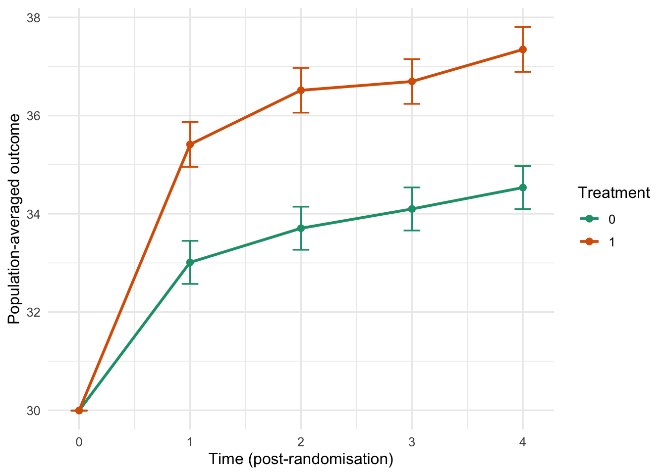
Population-averaged predictions with a common baseline
We can use marginaleffects::avg_predictions() to compute population-averaged curves by treatment arm and time, while forcing baseline to be the same for both groups. Here we set baseline to the overall mean baseline.
baseline_mean <- mean(dat$baseline)

newdata <- expand.grid(
  trt = c(0, 1),
  time_f = factor(times, levels = levels(dat$time_f)),
  baseline = baseline_mean
)

avg_predictions(
  raw_fit,
  newdata = newdata,
  by = c("trt", "time_f"),
  re.form = NA
)
##
##  trt time_f Estimate Std. Error   z Pr(>|z|)   S 2.5 % 97.5 %
##    0      1     33.0      0.224 148   <0.001 Inf  32.6   33.4
##    0      2     33.7      0.224 151   <0.001 Inf  33.3   34.1
##    0      3     34.1      0.224 152   <0.001 Inf  33.7   34.5
##    0      4     34.5      0.224 154   <0.001 Inf  34.1   35.0
##    1      1     35.4      0.233 152   <0.001 Inf  35.0   35.9
##    1      2     36.5      0.233 157   <0.001 Inf  36.1   37.0
##    1      3     36.7      0.233 158   <0.001 Inf  36.2   37.2
##    1      4     37.3      0.233 161   <0.001 Inf  36.9   37.8
##
## Type: response
library(ggplot2)

ap <- avg_predictions(
  raw_fit,
  newdata = newdata,
  by = c("trt", "time_f"),
  re.form = NA
)

ap0 <- data.frame(
  trt = c(0, 1),
  time_f = factor(0, levels = c(0, levels(dat$time_f))),
  estimate = baseline_mean,
  conf.low = baseline_mean,
  conf.high = baseline_mean
)

ap_plot <- rbind(
  transform(
    ap[, c("trt", "time_f", "estimate", "conf.low", "conf.high")],
    time_f = factor(time_f, levels = c(0, levels(dat$time_f)))
  ),
  ap0
)

ggplot(ap_plot, aes(x = as.numeric(as.character(time_f)), y = estimate, color = factor(trt), group = trt)) +
  geom_errorbar(aes(ymin = conf.low, ymax = conf.high), width = 0.15, linewidth = 0.6) +
  geom_line(linewidth = 1) +
  geom_point(size = 2) +
  scale_color_manual(values = c("0" = "#1b9e77", "1" = "#d95f02")) +
  scale_x_continuous(breaks = c(0, times)) +
  labs(
    x = "Time (post-randomisation)",
    y = "Population-averaged outcome",
    color = "Treatment"
  ) +
  theme_minimal(base_size = 12)
Why we use complex models: precision, not bias
In a properly randomized trial with complete follow-up data, a simple comparison of outcomes between groups (e.g., a t-test or linear regression with treatment only) is unbiased for the average treatment effect. The reason we use covariate adjustment and mixed models is primarily to improve precision and efficiency and to handle repeated measures and missing data under reasonable assumptions.
Take-home message
In repeated-measures RCTs with continuous outcomes:
- Treat baseline as a covariate, not an outcome.
- This respects the design (baseline is pre-randomization).
- It makes the model more flexible.
- It makes the change-from-baseline debate mostly irrelevant for inference.